LAB 2 Getting Started with R & Python

In this lab, we will start to go through some of the basic aspects of both R and Python. As this is the first real exposure for many of you, we will also get familiar with the RStudio IDE and the iPython notebook environments for doing data science.

R

R has emerged as among the most popular development environments for analytics. It has the advantage of being open source and free, has a great community, and it has a tremendous number of packages. As R is essentially a coding language specific to statistics, it has functional to do just about anything that you want to do.

Developing with R has made tremendous progress over a short period of time thanks to the developers at RStudio. RStudio is an Integrated Development Environment (IDE) for R that provides developers with an easy way to manage the development process. To use RStudio on the virtual machine, first make sure it is running (vagrant up to start).

Log onto the RStudio Sever (Virtual machine needs to be running) using the following.
http://localhost:8787
Username: vagrant
Password: vagrant

Once you log in you will be presented with the IDE console that has everything that you need to get started with data science.

title

When you launch RStudio Server, you immediately see view above. The R console provides a number of tools that can make data science quick and easy.

On the left side you can see the R console. The R console directly interprets R code and provides answers. Try it out by doing some basic math.

Math in R

3+3
20/4
20^2

Now assign the results to your first data structure the output of a calculation to a new variable.

n<-3+3

Notice that as you entered the variable into the R console, it showed up just to the top right of the screen. This provides a list of the objects available in memory. Just type n into the console again and get access to the variable and print it out.

Tip. Want to resubmit or slightly change a previous entry into the console? Just press up and then down in order to scroll through previous entries.

Programs (Scripts) in R.

While the console may allow you to quickly iterate and test commands, most times you are going to want to develop complex combinations of commands that can enable the transformation and analysis of data. Anything thing entered into the console is not persistant, meaning it is not saved past the initial session. As a result, we recommend working from a script. In reality, you can think of a script as a program that you are developing to complete some type of process. Start a new script now by File -> New File -> R Script.

Copy the earlier commands and add it directly to the script. You can then add comments to the script and save it for future use with the save button.

Scripts

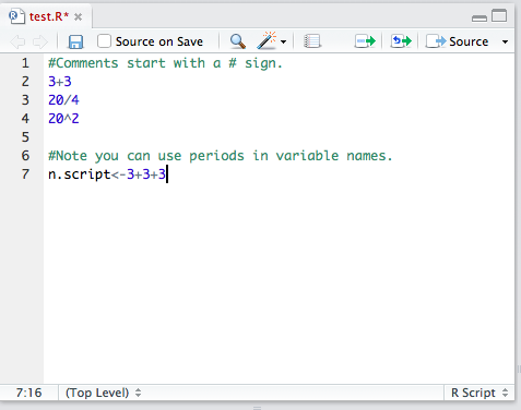
There are three different ways to execute the script.

The most common mode of operation is to highlight the code that you would like to execute and then press the execute (Run current line or selection). You can also do this using the shortcut key specific for Mac (command-Enter) or Windows (ctrl-enter).
After running a selection, you may find that you need to make an edit and rerun the same selection. The thoughtful individuals at RStudio have made this easy. Through the second execute button (Re-run the previous code region).
Finally, to execute the entire file, you can execute the source button (with echo to see it in the console).

R Vector

An R vector is a single set of values in a particular order of the same type. Even variables that we have set are really just array of length 1.

We can create a array using the concatenate function help(c) for more. Let’s say we want a vector with the ages for 4 students.

ages<-c(18,19,18,23)

To see this we can just type the name of object:

ages

To pick a specific value, we can, indicate it. Note. In some languages vectors will start at 0 while in R it will start with 1.

ages[4]

To specify the range of the vector, it can be clearly indicated.

ages[2:4]

We can have array of various types, and it is important to note that you cannot have data of 2 different types in the same array.

String. These are the clear character vectors. (Typically use quotes to add to these vectors.)
Numeric.Numbers in a set. Note there is not a different type
Boolean. TRUE or FALSE values in a set.
Factor. A situation in which there is a select set of options. Things such as states or zip codes. These are typically things which are related to dummy variables, a topic we will discuss later.

names<-c("Sally", "Jason", "Bob", "Susy") #Text
female<-c(TRUE, FALSE, FALSE, TRUE)
teachers<-c("Smith", "Johnson", "Johnson", "Smith")
teachers.f<-factor(teachers)
grades<-c(20, 15, 13, 19) #25 points possible

In each of the cases except factor, the default data provided by R was correct without direct specification. In the case of factor, the data needed to be explicitly cast as a factor vector.

Complete questions 1-3.

R Matrix

An R matrix is a 2 dimensional array that again must be of a single type. Here are several different ways of specifying a matrix.

#You can explicitly specify a matrix.
y<-matrix(1:10, nrow=3, ncol=3)

#Or you can put 2 single dimensional arrays together into a matrix.
mat <- matrix(cells, nrow=4, ncol=2, byrow=TRUE,
dimnames=list(students, teachers))
  
#Matrices can be specified by explicitly indicating the row and column, as follows. 
mat[2,1] #Row=2, Column=1
mat[1,]  #Row=1 and all columns 
mat[,1]  #Column=1, all rows

Matrix algebra is extremely useful in advanced statistics in which you are employing the underlying mathematical functions to do things like regression or to calculate properties of a network. However, in the majority of cases we will employ predefined functions in order to do analyses.

R List

A list is an array containing other R objects. While we won’t use it very frequently, it is a flexible data structure will contain the output of another analyses.

Unlike a vector or a matrix, a list can contain different data types.

x = list(names, female, teachers, grades) 
#This will call out the female vector.
x[2]
#This is a way of setting the first component of the list to false. There needs to be two brackets. 
x[[2]][1] = "FALSE"

R Dataframe

The data frame actually a special type of list, and it is the workhouse of the R analytics environment. The distinguishing factor of a data frame over a matrix is the ability to include different types of data. This means that you can mix numeric, string, boolean, etc. While R will default to the correct version in many cases, you also need to check that each field is coded correctly.

Let’s first look at a few different ways we can create data frames.

#This binds a data frame using a series of vectors. 
df1<-data.frame(cbind(names,teachers.f, teachers, ages, grades, percent))

#We can also load data from a csv file.  To load a file, we have to first tell R where to look by setting the active working directory.  
#This get set the working directory.
getwd()
#This will set the working directory.
setwd("/vagrant/data")
list.files()

#This names the file and pulls it into a data frame. 
titantic=read.csv(file="titantic_train.csv", header=TRUE,sep=",")

#Here are a variety of other operations you can do on a data frame. 
View(titantic) #show data browser
names(titantic) #show the names
dim(titantic) #show the dimensions of the data frame
head(titantic, 2) #show the first 2 records
tail(titantic, 4) #show the final 2 records
titantic$yearID #show the years in the data frame
summary(titantic) #summarize all variables
str(titantic) #shows the structure of an R Object

Using and defining functions in R

R has a wide array of functions that are predefined and can be used in the console. Before we look at R functions, let’s define are own so we understand how they work.

Let’s say we want a function that is ready to add 2 numbers. First we have to define the function.

#This defines a function called "addTwo."
addTwo <- function(a, b){
c<-a+b
return(c)
}

By selecting this function and running it, we can now have access to the function in memory for the rest of this R session. If we open the script again we would again have to go through the process of loading the function into memory.

We can then go through the process of utilizing the function by calling it and then specifying the two associated parameters a & b.

addTwoNumbers(4, 5)

Note that the function specification and use is case sensitive. The use of descriptive functions with all words except the first capitalized in known as camel case.

Organizing processing of data into functions is quite convenient and facilitates what is one of the holy grails of programming: code reuse. By organizing processing of data into functions, you can easily process data for different datasets or subsets of the data without rewriting the steps for each.

There are lots of built in functions in R that can provide important functionality. Run the following and see:

#Here are some misc.
x<-abs(-20)
textfield<-toupper("this is a lowercase sentence")

To understand each function, we can use the embedded help function help(abs) to find out about the absolute value function and help(toupper) to find out about the to uppercase function.

We can also apply functions to vectors to generate other variables and vectors.

grades.sum<-sum(grades)
grades.sum
names.length<-nchar(names) 
names.length

Control Structures

There are many cases where you want to control the flow of a program, introducing conditionals or loops. R has a number of different options for this.

grade<-function(a){
  if(a>90) {
    grade<-"A"  }
  else if (a >80) {
    grade<-"B" }
  else {
    grade<-"P"
  }    
  return (grade)
}

x <- 85
mygrade<-grade(x)
mygrade
percent<-(grades/25*100)
len<-length(percent)
len

lettergrade <- character(len)

#This for loop will progress over the array, executing the function for each.  
for (n in 1:len)
{
  lettergrade[n]<-grade(percent[n])
}

That is all for now. Let’s start looking at some basic data in Python.

Python

When learning different languages, it is useful to map concepts. In this case we will be going through the process of learning similar concepts in python that we have just learned in R. The hope is that you will both be able to be fluent in more than one language and gain a better understanding of the underlying concepts.

To access iPython, you just need to access another port of your localhost. Localhost is your machine, and Vagrant has done an excellent job of mapping the ports on your machine (that is the 8001 below) to the appropriate port on the virtual machine.
http://localhost:8001

The virtual machine is configured with Jupyter, a tool that evolved from the iPython notebook. You see, a lot of people realized that the specific form of embedding HTML and code that makes up iPython notebooks, can also be useful for a number of other languages. Jupyter enables use with Python, Julia, R, Haskell, or Ruby. We will just be using Python in our in initial work.

There are a tremendous wealth of tutorials out there that give you the basics of Python. Data science is quite different from application building through, necessitating not different understanding but different applications.

The iPython environment is transitioning to Jupyter, as the notebook style of model has been found to be an extremely valuable method of doing data science that has relevance for other languages like R. In our current VM, we only have the python engine installed, but this area is moving quickly and things are converging quickly.

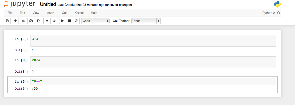
In iPython, each cell represents a separate input of code. For example, to complete each of these separate operations they need to be put in three separate cells.

Math in Python

3+3
20/4

#Note this is a bit different than R.  While R uses a "^", python uses "**" to indicate an exponent.
20**2

title

Now assign the results to your first data structure the output of a calculation to a new variable.

n=3+3
print n

In the specification above, note that we use the = to specify a variable in python while in R we used <-. We also had to explicitly specify the output via print while the R console just threw it back at us.

Tip. Want to resubmit or slightly change a previous entry into the console? Just press up and then down in order to scroll through previous entries.

Programs (Scripts) in Python.

While the cell may allow you to quickly iterate and test commands, most times you are going to want to develop complex combinations of commands that can enable the transformation and analysis of data, as we did in R.

The Jupyter notebook provides a wide number of options to run the cells in different ways.
title

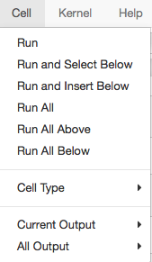
For the most part these different methods are self explanatory. In my case, I find that the majority of the time I will run just the current cell, run all cells, or run the cells above. While a notebook provides a useful framework to run a series of commands.

Python Arrays

As in R, a with Python we need ways of doing complex operations of vectors and matrixes. Unlike R, there are different models for doing this. As data structures are objects, they inherit their properties from the underlying classes that define them.

Let’s start with the basic list. This is an ordered collection of objects that can be of any type.

#To start with, let's define lists.
names=["Sally", "Jason", "Bob", "Susy"]
#Note that the the all caps we used for R won't work for Python!
female=[True, False, False, True]
teachers=["Smith", "Johnson", "Johnson", "Smith"]
ages =  [18,19,18,23] 
grades= [20, 15, 13, 19]
print names
print female
print ages
print grades


#To pick a specific value, we can, indicate it. *Note. In Python vectors will start at 0 while in R it will start with 1.* 
 
ages[3]


#To specify the range of the array, the numbering is a bit different.  

print ages[1:3]

The list module embedded in Python is fine for temporarily storying data, but to do operations on it we would like to use the numpy package. While we haven’t gone over packages yet, this is a way of implementing new functionality. NumPy is one of the foundational packages for the data scientist using python. It includes a powerful N-dimensional array object, which you can think of like a more flexible version of the R array. Numpy, like R also has different data types, but they are even more extensive in their options.

Here are some more common ones:

str These are the clear character vectors. (Typically use quotes to add to these vectors.)
int_Integer
bool_ True or False values in a set.

And you can view the entire list here.

import numpy as np
namesNP=np.array(names) 
femaleNP=np.array(female)
teachersNP=np.array(teachers)
gradesNP=np.array(grades)

#You can then change the type.
gradesNP.astype(np.int32)

#Alternately you can directly specify the type
import numpy as np
namesNP=np.array(names, np.string_) 
femaleNP=np.array(female, np.bool_)
teachersNP=np.array(teachers, np.string_)
agesNP=np.array(ages,  np.int32)
gradesNP=np.array(grades, np.int32)

Doing operations on NP arrays is a bit different than in R, and it requires the use of specific functions. Her are two ways we can multiply an array. Here we are really calling a method for completing the desired functionality. Here you can see a variety of the math related functions available.

# Multiply
percentNP2=np.multiply(gradesNP, 4)
print percentNP2

percentNP=np.array(np.multiply(grades, 4))
print percentNP

print agesNP
agesNP=np.add(agesNP, 1)
print agesNP

ageNP=np.add(ageNP, 1)

Python Matrix

An Python matrix has two dimensions and has similar properties of an R matrix. Most important is that multidimensional arrays have to be of a single type. Lets first look at what happens when we mix types.

alldata=np.array([names, female, teachers, ages, grades])
alldata2=np.array([namesNP, femaleNP, teachersNP, agesNP, gradesNP])
somedata=np.array([agesNP, gradesNP])

print alldata
print alldata2 
print somedata
  
#Matrices can be specified by explicitly indicating the row and column, as follows. 
print alldata[2,1] #Row=2, Column=1
print alldata[1,]  #Row=1 and all columns 
print alldata[,1]  #Column=1, all rows

Python Dataframe with Pandas

Like in R, in Python we need a way of mixing data of a variety of different types together for analysis. Pandas to the rescue. Pandas is a powerful Python package that can be used for a wide variety of operations, and we will use it as a foundation for many of our data structures.

It is also, however, one that I neglected to install in the original image. Let’s go through the process of installing a python Package.

The most consistent way of installing a Python package is directly on the server via a command line. The Python package manager takes care of almost all of the complexity.

Log into the virtual machine with vagrant ssh. This brings you into the server. Then just install Pandas via sudo pip install pandas. This will download and install the Pandas and any other requirements.

Let’s first look at a few different ways we can create data frames. The one for data below is a build in Python data structure called a dict that provide a dictionary that can be used to look up values. In some other languages they are called hashes.

from pandas import Series, DataFrame
import pandas as pd

data = { 'names': ['Sally', 'Jason', 'Bob', 'Susy'],
               'female': [True, False, False, True],
               'ages':  [18,19,18,23] ,
               'grades': [20, 15, 13, 19]}
               
alldataDF = DataFrame(data, columns=['names', 'female', 'ages', 'grades'])

#this can print out all of the data 
alldataDF

#This will present just the names. 
alldataDF['names']

#Now let's read in our titanic dataset.
titanticDF = pd.read_csv('/vagrant/assets/data/ti')
titanticDF

#If that didn't work, it probably means that the sharing between your host and virtual machine are not working.  You pay want to install an older version of virtual box (4.3.10) and try rebuilding the machine.  Otherwise you can for now pull the file from online.

import csv
import urllib2

url = 'https://raw.githubusercontent.com/RPI-Analytics/MGMT6963-2015/master/data/titantic_train.csv'
response = urllib2.urlopen(url)
cr = pd.read_csv(response)
cr

We can execute commands on the server through iPython.

!cd /vagrant/data
!ls

You can download some excellent ipython notebooks here that cover some of the basics of data frames. This is high quality material and you should go through Chapters 1-3.

Using and defining functions in Python

Just like R, Python has a way to embed functions. What is a bit different about Python is how it uses spaces to specify the start and end of the functions. While it is possible to use tabs or different levels of indentation, the (PEP 0008 style guide) for Python recommends 4 spaces indentation.

Let’s say we want a function that is ready to add 2 numbers. First we have to define the function.

#This defines a function called "addTwo."
def addTwoNumbers( a, b ):
    c=a+b  
    return c;

By selecting this function and running it, we can now have access to the function in memory for the rest of this Python session. If we open the script again we would again have to go through the process of loading the function into memory.

We can then go through the process of utilizing the function by calling it and then specifying the two associated parameters a & b.

addTwoNumbers(4, 5)

There are lots of [built in functions] in Python that can provide important functionality.

x=abs(-20)
print x

sentence= "this is a lowercase sentence"
sentence.upper()
print sentence

Here we are running a specific method (upper) that is a property of the underlying class of a string. This is a little bit different than how we did things in R (passing a variable to a function), but it is extremely efficient.

Controls in Python

We have lots of options for control of programs in Python. Read here for some examples.

#while in R we use {} to specify for loops, in Python we just use the indentation.  Remember, 4 spaces
for n in grades:
    print grades[n]

Lab Questions
All work should be your own. Please write the answers to these questions in a word file and upload to Blackboard.

What happens when we mix types in R?
age<-c(20, 15, 13, “ten”)
Can you do math on vectors in R? Try the following. What happens and why? [Uses code from above.
percent<-(grades/25*100)
age<-age+1
In completing this challenge, you should do it in class.
Using R, Write a set of commands that returns the sum, average, and standard deviation of a vector.
Using R, write a set of commands that swaps a set of variables such that A is equal to B and B is equal to A.
Describe the difference between a factor vector and a String vector in R.
Think back to our Titanic dataset. Could we employ an R matrix for this data? Why or why not?
In R, why is it relevant to set the working directory? On the virtual machine, what directory corresponds with the course repository?
Specify the R code to do each of the following: (a.) a random number between 1 and 8. (b.) a random integer between 1 and 10. (c.) a random set of 2 integers 1-10 that are not the same, (d.) a random number from a distribution with a mean of 4 and a standard deviation of 2.
**Hint: This guide and this guidecan provide a nice overview.
What does it mean to sample random numbers “with replacement” vs. without replacement.
Is there a difference between the data stored via the alldata and the alldata2 array in the above Python example? Why?
Is there a difference with the somedata versions of ages/grades and the all data version of ages/grades in the Python example?
Create a function in R that accepts 2 value (n, m) and returns an N x M matrix with random numbers with a mean of 20 and a standard deviation of 5.
Write Python code to set a variable n equal to 144 and then take the square route of n.
Using Python, write a set of commands that swaps a set of variables such that A is equal to B and B is equal to A. [For example, let’s say A = 5 and B = 6 at the beginning. After entering your commands A must be equal to 6 and B must be equal to 5.]
Describe how the subsetting of arrays works differently in Python than R. For example, how would grades[2] and grades[3:4] work differently in R and Python.
Create a function which returns an array of 2 different strings from a character array. Hint. If given, a character array such as names, where….names=[“Sally”, “Jason”, “Bob”, “Susy”] The function should (randomly) return 2 of the names. For example, [‘Sally’, ‘Susy’].
Find a different CSV from the classroom discussion and upload it to a Pandas. Was the data processed correctly?

Images Credits

Matrix
https://commons.wikimedia.org/wiki/File%3AMatrix.svg
By Lakeworks (Own work) [GFDL (http://www.gnu.org/copyleft/fdl.html) or CC BY-SA 4.0-3.0-2.5-2.0-1.0 (http://creativecommons.org/licenses/by-sa/4.0-3.0-2.5-2.0-1.0)], via Wikimedia Commons

##Lab 2 Solution.
1. What happens when we mix types in R?
age<-c(20, 15, 13, “ten”)

You cannot mix numeric variables with text. The entire vector is treated as text

Can you do math on vectors in R? Try the following. What happens and why? [Uses code from above.]
percent<-(grades/25*100)
age<-age+1
You can do math on vectors but in the above example, age is treated as a string vector.
Using R, write a set of commands that returns the sum, average, and standard deviation of a vector.

ages<- c(19,19,12,23)
ages.sum<- sum(ages)
ages.mean<-mean(ages)
ages.sd<-sd(ages)

Using R, write a set of commands that swaps a set of variables such that A is equal to B and B is equal to A.

a<-4
b<-3
c<-a
a<-b
b<-c

Describe the difference between a factor vector and a String vector in R.

“Factor variables are categorical variables that can be either numeric or string variables. There are a number of advantages to converting categorical variables to factor variables. Perhaps the most important advantage is that they can be used in statistical modeling where they will be implemented correctly, i.e., they will then be assigned the correct number of degrees of freedom.” Source

Think back to our Titanic dataset. Could we employ an R matrix for this data? Why or why not?

No, because the data was of many different types.

In R, why is it relevant to set the working directory? On the virtual machine, what directory corresponds with the course repository?

Setting the working directory provides a location of the files. This is where R will look for a file. Files between the guest and the host will be shared at /vagrant.

Specify the R code to do each of the following: (a.) a random number between 1 and 8. (b.) a random integer between 1 and 10. (c.) a random set of 2 integers 1-10 that are not the same, (d.) a random number from a distribution with a mean of 4 and a standard deviation of 2.
**Hint: This guide and this guidecan provide a nice overview.

# A. A random number between 1 and 8. 
x1 <- runif(1, 1, 8)
x1 

# B. A random integer between 1 and 10.
 x2 <- sample(1:10, 1)
 x2
 
 # C. A random set of 2 integers 1-10 that are not the same
x3 <- sample(1:10, 2, replace=F)
x3

# D. A random number from a distribution with  a mean of 4 and a standard deviation of 2. 
x4 <- rnorm(5, mean=4, sd=2)
x4

What does it mean to sample random numbers “with replacement” vs. without replacement.

With replacement means random numbers can repeat. Without replacement means that the random numbers cannot repeat.

Is there a difference between the data stored via the alldata and the alldata2 array in the above Python example? Why?

No difference between the two arrays.

Is there a difference with the somedata versions of ages/grades and the all data version of ages/grades in the Python example?

Yes - because all data in a numpy array has to be of a single type, the alldata version of ages/grades are characters because namesNP, femaleNP, and teachersNP are character/string. The somedata version of ages/grades are numeric/integer type (no single quotes).

Create a function in R that accepts 2 value (n, m) and returns an N x M matrix with random numbers with a mean of 20 and a standard deviation of 5.

n <- sample(1:9, 1)
m <- sample(1:9, 1)
test1 <- function(n,m) {matrix(rnorm(n*m, mean=20, sd=5), nrow=n, ncol=m)}
test1(n,m)

Write Python code to set a variable n equal to 144 and then take the square route of n.

import math
	n = 144
	math.sqrt(n)

Using Python, write a set of commands that swaps a set of variables such that A is equal to B and B is equal to A. [For example, let’s say A = 5 and B = 6 at the beginning. After entering your commands A must be equal to 6 and B must be equal to 5.]

var1 = 2
	var2 = 4
	var1 = var1 + var2
	var2 = var1 - var2
	var1 = var1 - var2
	print var1
	print var2

Describe how the subsetting of arrays works differently in Python than R. For example, how would grades[2] and grades[3:4] work differently in R and Python.

With grades = [20, 15, 13, 19)
	in R - grades[2] returns the 2nd value (15) in the array
	in Python - grades[2] returns the 3rd value (13) in the array
	**because Python indexing starts at 0 and R indexing starts at 1
	in R - grades[3:4] returns (13, 19)
	in Python - grades [3:4] returns (19)
	**because a subset in Python does not include the final element in the slice (i.e. the “4” in 3:4)

Create a function which returns an array of 2 different strings from a character array. Hint. If given, a character array such as names, where….names=[“Sally”, “Jason”, “Bob”, “Susy”] The function should (randomly) return 2 of the names. For example, [‘Sally’, ‘Susy’].

test1 = ["red","orange","yellow","green","blue","indigo","violet"]
	def split():
    		return [random.choice(test1), random.choice(test1), random.choice(test1)], [random.choice(test1), random.choice(test1), random.choice(test1)]
	arr1, arr2 = split()
	print arr1
	print arr2

Find a different CSV from the classroom discussion and upload it to a Pandas. Was the data processed correctly?